7.01 Covering spaces
Below the video you will find accompanying notes and some pre-class questions.
- Next video: 7.02 Path-lifting, monodromy.
- Index of all lectures.
Notes
Intuition for covering spaces
(0.30) Take \(\mathbf{C}\setminus\{0\}\) and consider the map
\(p\colon\mathbf{C}\setminus\{0\}\to\mathbf{C}\setminus\{0\}\) given
by \(p(z)=z^2\). This map is surjective and 2-to-1. Nonetheless, we
do have something like an inverse locally: the square root function
(we actually have two local inverses differing by a sign
\(\pm\sqrt{}\)).
(4.00) We could equally have taken a branch cut
\(\{z\in\mathbf{C}\setminus\{0\}\ :\ Im(z)=0,\ Re(z)>0\}\) and we
would have obtained two different local inverses for \(p\). The point
of taking a branch cut is that \(\mathbf{C}\setminus\{0\}\) is not
simply-connected but \(\mathbf{C}\setminus B\) is simply-connected,
which is what lets us define an inverse on the complement of the
branch-cut.
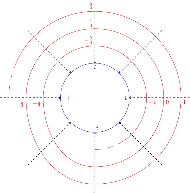
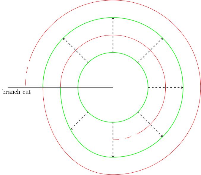
(2.26) More precisely, if we excise a half-line \(B=\{z\in\mathbf{C}\setminus\{0\}\ :\ Im(z)=0,\ Re(z)<0\}\) then on \(\mathbf{C}\setminus B\) we have two functions \[q_+,q_-\colon\mathbf{C}\setminus B\to\mathbf{C}\setminus\{0\}\] such that \(p(q_\pm(z))=z\). In this example, \(q_-=-q_+\), e.g.\(q_+(1)=1\), \(q_-(1)=-1\).
(5.11) Take \(f\colon\mathbf{C}\mapsto\mathbf{C}\setminus\{0\}\),
\(f(z)=e^{iz}\). This map is surjective and \(\infty\)-to-1 (for
example \(f^{-1}(1)=\{2\pi n\ :\ n\in\mathbf{Z}\}\)). On the
complement of a branch cut \(B\) we have infinitely many
well-defined local inverses \(q_n=2\pi
n-i\log)\colon\mathbf{C}\setminus B\to\mathbf{C}\) satisfying
\(q_n(1)=2\pi n\) and \(p(q_n(z))=z\) (that is \(\exp(i(2\pi n-i\log
z))=z\)). [The video is missing a factor of \(-i\).]
(9.00) Roughly speaking, a covering map is a map \(p\colon Y\to X\)
which is \(N\)-to-1 for some \(N\) and which has \(N\) locally-defined
inverses \(q_n\) defined on simply-connected subsets of the target
(satisfying \(p\circ q_n=id\)).
(10.40) Notice that in the second example, the domain of the
covering map is \(\mathbf{C}\), which is simply-connnected, and the
local inverses \(q_n\) are indexed by the integers
\(\mathbf{Z}\). This is, roughly speaking, how you deduce that the
target of the covering map has \(\pi_1\cong\mathbf{Z}\).
Definition
(11.20) Let \(p\colon Y\to X\) be a continuous map.
(18.36) Here is a picture of the exponential map \(p(z)=e^{iz}\)
restricted to the real axis (so its image is the unit circle in
\(\mathbf{C}\)):
- A subset \(U\subset X\) is called an elementary
neighbourhood if there is a discrete set \(F\) and a
homeomorphism \(h\colon p^{-1}(U)\to U\times F\) such that
\(pr_1\circ h=p|_{p^{-1}(U)}\) (where \(pr_1\colon U\times F\to
U\) is the projection to the first factor).
- (13.30) You should think of an elementary neighbourhood as playing the role of the complement of a branch cut in our earlier examples: \(U\) is the subset on which you have locally-defined inverses to \(p\).
- (13.57) The locally-defined inverses are parametrised by the discrete set \(F\); in our examples we had \(F=\{-1,1\}\) and \(F=\mathbf{Z}\). For each point \(m\in F\) we get a map \(q_m\colon U\to U\times F\to p^{-1}(U)\) defined by \(q_m(x)=h^{-1}(x,m)\) which satisfies \(p(q_m(x))=pr_1(h(h^{-1}(x,m)))=x\).
- (16.07) We say \(p\) is a covering map if \(X\) is
covered by elementary neighbourhoods (i.e. every point \(x\in X\)
is contained in some elementary neighbourhood).
- Note that the word cover can now mean two things: covering map and open cover (like in the definition of compactness). Hopefully it will be clear what is meant from the context.
- (17.40) We say that a subset \(V\subset Y\) is an
elementary sheet if it is path-connected and \(p(V)\) is an
elementary neighbourhood.
More examples
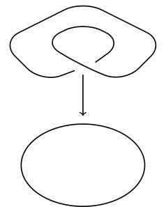
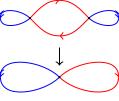
(24.05) Consider the figure 8, with its two loops drawn in red and
blue. The following picture defines a 2-to-1 covering space of the
figure 8:
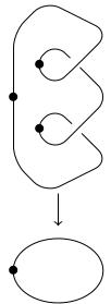
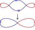
(26.22) Another covering space of the figure 8 is given by this
picture:
Pre-class questions
- Are there any other 2-to-1 covers of the figure 8? Remember, in each
case, the cross-point has two preimages which look like
cross-points, each edge has two preimages which connect the
cross-points.
Navigation
- Next video: 7.02 Path-lifting, monodromy.
- Index of all lectures.