Chain relations

There is a beautiful series of relations in the mapping class groups of punctured surfaces called the chain relations. In this post, I will explain the origin of these relations in algebraic geometry.

The relations

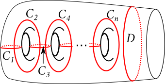
If \(n\) is even, the \(n\)-chain relation tells us that \[(\tau_{C_1}\cdots\tau_{C_n})^{2n+2}=\tau_{D}\] where \(\tau_A\) denotes the right-handed Dehn twist in the curve \(A\) and \(C_1,\ldots,C_n,D\) are as shown below.

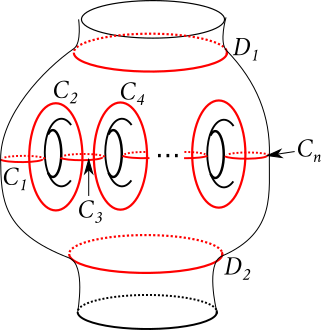
If \(n\) is odd, the \(n\)-chain relation tells us that \[(\tau_{C_1}\cdots\tau_{C_n})^{n+1}=\tau_{D_1}\tau_{D_2}\] for the curves shown below.

I recently realised that there's a nice algebro-geometric proof of these relations, which had formerly been somewhat mysterious to me.

The proof

We'll focus on the \(n\)-even case first.

Right hand side

Consider the surface \(X\subset\mathbf{C}^3\) defined by the equation \(x^2+y^{n+1}+z^{2(n+1)}=0\). This surface has an isolated singularity at the origin. Let \(f\colon\tilde{X}\to X\) be the minimal resolution. The exceptional locus is a smooth, irreducible curve of genus \(n/2\). I will justify this below.

Next, consider the projection to the \(z\) coordinate \(z\colon X\to\mathbf{C}\). This is a holomorphic map; its fibres are \(\{x^2+y^{n+1}=-z^{2(n+1)}\}\) which are smooth copies of the \(A_n\)-Milnor fibre if \(z\neq 0\). This Milnor fibre is the curve shown in the figure for the \(n\)-chain relation (i.e. a once-punctured curve of genus \(n/2\)). The fibre over \(z=0\) is the singular curve \(x^2+y^n=0\). This has a single branch passing through the origin, and its proper transform is a smooth copy of \(\mathbf{C}\) which hits the exceptional locus at a single point.

The composition \(z\circ f\colon\tilde{X}\to\mathbf{C}\) is now a holomorphic map whose fibres are:

• the smooth \(A_n\)-Milnor fibre over \(z\neq 0\),
• a plane with a curve of genus \(n/2\) attached at the origin over \(z=0\).

This central fibre is obtained from the smooth fibre by collapsing a boundary-parallel loop, i.e. the simple closed curve \(D\). The monodromy of this fibration is the Dehn twist around \(D\), i.e. the right hand side of the \(n\)-chain relation.

Left hand side

Consider the smoothing \(X_\epsilon=\{x^2+y^n+z^{2n}=\epsilon\}\) of \(X\) for \(\epsilon\neq 0\). Again, projecting \(X_\epsilon\) \(z\)-coordinate we get a holomorphic fibration \(f_\epsilon\colon X_\epsilon\to\mathbf{C}\) and the monodromy around the unit circle has not changed (up to isotopy) provided \(\epsilon\) is small enough, so whatever we get will be isotopic to \(\tau_D\).

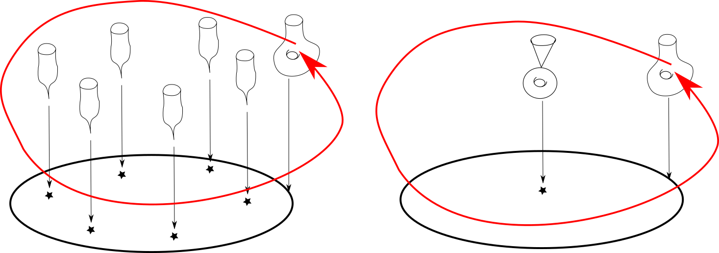
The fibration \(f_\epsilon\) has \(2(n+1)\) singular fibres at the points where \(z^{2(n+1)}=1\). Each of these singular fibres (\(x^2+y^n=0\), \(z\) fixed) has a single \(A_n\)-singularity. If we pick a vanishing path \(\gamma\) in the base which connects \(z=1\) to \(z=0\) then the vanishing cycle is precisely the \(A_n\)-chain in the smooth fibre over zero. If we apply the automorphism \((x,y,z)\mapsto (x,y,\mu z)\) (where \(\mu^{2(n+1)}=1\)) then we get the same vanishing cycle for the vanishing paths \(\mu^k\gamma\) (because the vanishing cycle lives in \(z=0\), which is fixed by the automorphism). The monodromy for this fibration is therefore \(\tau^{2(n+1)}\) where \(\tau\) is the monodromy for the \(A_n\)-chain (which, it is easy to check, is the product \(\tau_{C_1}\ldots\tau_{C_n}\)).

This implies the chain relation when \(n\) is even. The picture below attempts to illustrate the case \(n=2\). The two red arrows indicate the monodromies (which are the same in each picture). The six singular fibres on the left are obtained by collapsing an \(A_2\)-chain in the smooth fibre.

\(n\) odd

When \(n\) is odd, we run the same argument with the variety \(X=\{x^2+y^{n+1}+z^{n+1}=0\}\) (the exceptional locus of the minimal resolution is now a smooth curve of genus \((n-1)/2\) and the normalisation of the fibre \(x^2+y^{n+1}=0\) has two components, so we get two boundary twists).

The minimal resolution

I want to justify why the minimal resolution of \(x^2+y^{n+1}+z^{2(n+1)}\) (\(n\) even) is what I say it is. Make a weighted blow-up at the origin with weights \(n+1,2,1\), that is consider the surface \[\tilde{X}=\{(x,y,z,[a:b:c])\in \mathbf{C}^3\times\mathbf{P}(n+1,2,1)\ :\ x^2+y^{n+1}+z^{2(n+1)}=0,\ \mbox{Plucker}\}\] where Plücker stands for the three relations \(xb=ay,xc=az,yc=bz\) which become \([a:b:c]=[x:y:z]\) if \((x,y,z)\neq(0,0,0)\). Here \(\mathbf{P}(n+1,2,1)\) is the weighted projective space \(\operatorname{Proj}(\mathbf{C}[a,b,c])\) where \(a,b,c\) are given degrees \(n+1,2,1\) respectively. The projection \(f\colon\tilde{X}\to X\) gives the minimal resolution of \(X\) and the exceptional locus of \(f\) is the curve \(\{x^2+y^{n+1}+z^{2(n+1)}=0\}\subset\mathbf{P}(n+1,2,1)\) which is a smooth curve of genus \(n/2\) (for background on weighted projective spaces, see [Reid], [Iano-Fletcher], [Dolgachev], [Hosgood]; the last two references explain ways to compute the genus of a smooth weighted plane curve [Dolgachev, Section 3.5.2], [Hosgood, Theorem 3.5.7]).

References

[Dolgachev] Dolgachev, I. Weighted projective varieties, (1982), in Group actions and vector fields (Vancouver, B.C., 1981), Lecture Notes in Math., 956, Berlin: Springer, pp. 34-71 available from Dolgachev's website and from Springer with DOI: https://doi.org/10.1007/BFb0101508.

[Hosgood] Hosgood, T. An introduction to varieties in weighted projective space, (2016) arXiv:1604.02441

[Iano-Fletcher] Working with weighted complete intersections, in Explicit birational geometry of 3-folds, A. Corti and M. Reid (Editors) CUP 2000. Available from Reid's website in PostScript format and from CUP with DOI: https://doi.org/10.1017/CBO9780511758942.005

[Reid] Reid, M. Graded rings and varieties in weighted projective space. (2002) available from Reid's website.