34. Eigenspaces

0.00 In all the examples we've seen so far, the eigenvectors have all had a free variable in them. For example, in the last video, we found the eigenvectors for the matrix $A=\begin{pmatrix}\frac{3}{2}&\frac{5}{2}&3\\ -\frac{1}{2}&-\frac{3}{2}&-3\\ 1&1&2\end{pmatrix}$ to be:

for $\lambda=1$ , $\begin{pmatrix}x\\ -5x\\ 4x\end{pmatrix}$ ,
for $\lambda=2$ , $\begin{pmatrix}x\\ -x\\ 0\end{pmatrix}$ ,
for $\lambda=-1$ , $\begin{pmatrix}x\\ -x\\ x\end{pmatrix}$

For the matrix $\begin{pmatrix}2&1\\ 1&1\end{pmatrix}$ we found the eigenvalue $\frac{3\pm\sqrt{5}}{2}$ had eigenvectors $\begin{pmatrix}x\\ \frac{-1\pm\sqrt{5}}{2}x\end{pmatrix}$ . All of these have the free parameter $x$ .

0.48 This is a general fact:

Lemma:

If $v$ is an eigenvector of $A$ with eigenvalue $\lambda$ ("a $\lambda$ -eigenvector") then so is $k v$ for any $k\in\mathbf{C}$ .

$A(kv)=kAv=k\lambda v=\lambda(kv)$ .

2.08 So for example, the vectors $\begin{pmatrix}x\\ -x\\ x\end{pmatrix}$ are all just rescalings of $\begin{pmatrix}1\\ -1\\ 1\end{pmatrix}$ . Indeed, people often say things like "the eigenvector is $\begin{pmatrix}1\\ -1\\ 1\end{pmatrix}$ ", when they mean "the eigenvectors are all the rescalings of $\begin{pmatrix}1\\ -1\\ 1\end{pmatrix}$ ". If you write this kind of thing in your answers, that's fine.

Example:

3.26 Suppose we have the matrix $I=\begin{pmatrix}1&0\\ 0&1\end{pmatrix}$ . The characteristic polynomial is $\det(I-\lambda I)=\det\begin{pmatrix}1-\lambda&0\\ 0&1-\lambda\end{pmatrix}=(1-\lambda)^{2}$ , so $\lambda=1$ is the only eigenvalue. Any vector $v$ satisfies $Iv=v$ , so any vector $\begin{pmatrix}x\\ y\end{pmatrix}$ is a $1$ -eigenvector. This has two free parameters, so it is an eigenplane, not just an eigenline: there is a whole plane of eigenvectors for the same eigenvalue.

Theorem:

4.45 The set of eigenvectors with eigenvalue $\lambda$ form a (complex) subspace of $\mathbf{C}^{n}$ (i.e. closed under complex rescalings and under addition).

5.29 Let $V_{\lambda}$ be the set of $\lambda$ -eigenvectors of $A$ . If $v\in V_{\lambda}$ then $kv\in V_{\lambda}$ (as we saw above). If $v_{1},v_{2}\in V_{\lambda}$ then $A(v_{1}+v_{2})=Av_{1}+Av_{2}=\lambda v_{1}+\lambda v_{2}=\lambda(v_{1}+v_{2}),$ so $v_{1}+v_{2}$ is also a $\lambda$ -eigenvector.

6.47 We call this subspace the $\lambda$ -eigenspace. In all the examples we saw earlier (except $I$ ), the eigenspaces were 1-dimensional eigenlines (one free variable). So a matrix gives you a collection of preferred directions or subspaces (its eigenspaces), which tell you something about the matrix (e.g. if it's a rotation matrix, its axis will be one of these subspaces).

Example:

8.42 For the example $A=\begin{pmatrix}2&1\\ 1&1\end{pmatrix}$ we found the eigenvalues $\frac{3\pm\sqrt{5}}{2}$ and eigenvectors $\begin{pmatrix}x\\ \frac{-1\pm\sqrt{5}}{2}x\end{pmatrix}$ . We now draw these two eigenlines (in red).

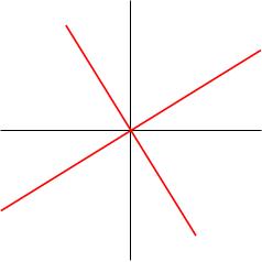
10.39 Note that these eigenlines look orthogonal; indeed, you can check that they are! You do this by taking the dot product of the eigenvectors (it's zero). This is true more generally for symmetric matrices (i.e. matrices $A$ such that $A=A^{T}$ ).