37. Eigenapplications, 3: Dynamics

0.00 We now turn to dynamics. Let $v$ be a vector and $A$ be a matrix. Consider the sequence $v,Av,A^{2}v,A^{3}v,\ldots$ . We'll investigate what happens to this sequence $A^{n}v$ as $n\to\infty$ .

Example: Fibonacci sequence

0.42 Let $A=\begin{pmatrix}0&1\\ 1&1\end{pmatrix}$ and $v=\begin{pmatrix}1\\ 1\end{pmatrix}$ . We get $Av=\begin{pmatrix}1\\ 2\end{pmatrix},\qquad A^{2}v=\begin{pmatrix}2\\ 3\end{pmatrix},\qquad A^{3}v=\begin{pmatrix}3\\ 5\end{pmatrix},\qquad A^{4}v=\begin{pmatrix}5\\ 8\end{pmatrix},$ and, more generally, $A^{n}v=\begin{pmatrix}F_{n}\\ F_{n+1}\end{pmatrix}$ where $F_{0}=1$ , $F_{1}=1$ , $F_{2}=2$ , $F_{3}=3$ , $F_{4}=5$ , $F_{5}=8$ , $F_{6}=13$ is the Fibonacci sequence.

2.27 Why are we getting the Fibonacci numbers? Suppose the formula $A^{n}v=\begin{pmatrix}F_{n}\\ F_{n+1}\end{pmatrix}$ is true for some value of $n$ ; we'll prove it's true for all values of $n$ by induction: $A^{n+1}v=AA^{n}v=A\begin{pmatrix}F_{n}\\ F_{n+1}\end{pmatrix}=\begin{pmatrix}F_{n+1}\\ F_{n}+F_{n+1}\end{pmatrix}=\begin{pmatrix}F_{n+1}\\ F_{n+2}\end{pmatrix},$ where we used the recursive formula $F_{n+2}=F_{n+1}+F_{n}$ which defines the Fibonacci sequence.

3.20 As $n\to\infty$ , both entries of the vector tends to infinity, but they do so in a particular way:

Theorem:

We have $\lim_{n\to\infty}\frac{F_{n+1}}{F_{n}}=\frac{1+\sqrt{5}}{2}.$ This expression is the "golden ratio" $1.618\cdots$ .

4.09 Write $v=\begin{pmatrix}1\\ 1\end{pmatrix}$ as $\alpha u_{1}+\beta u_{2}$ where $u_{1}$ and $u_{2}$ are the $\lambda_{1}$ - and $\lambda_{2}$ -eigenvectors of $A=\begin{pmatrix}0&1\\ 1&1\end{pmatrix}$ . We'll figure out what these eigenvectors and eigenvalues are later.

5.08 Now $A^{n}v=A^{n}(\alpha u_{1}+\beta u_{2})=\alpha A^{n}u_{1}+\beta A^{n}u_{2}$ . We have $Au_{1}=\lambda_{1}u_{1}$ , $A^{2}u_{1}=\lambda_{1}Au_{1}=\lambda_{1}^{2}u_{1}$ , and by induction we get $A^{n}u_{1}=\lambda_{1}^{n}u_{1},\qquad A^{n}u_{2}=\lambda_{2}^{n}u_{2}.$ 6.04 Therefore $\begin{pmatrix}F_{n}\\ F_{n+1}\end{pmatrix}=A^{n}v=\alpha\lambda_{1}^{n}u_{1}+\beta\lambda_{2}^{n}u_{2}$ .

6.40 I claim that $\lambda_{1}=\frac{1+\sqrt{5}}{2}\approx 1.618\cdots$ and $\lambda_{2}=\frac{1-\sqrt{5}}{2}\approx-0.618\cdots$ . Therefore:

$\lambda_{1}>1$ , so $\lambda_{1}^{n}\to\infty$ ,
$\lambda_{2}^{n}\to 0$ as $n\to\infty$ . Note that $\lambda_{2}$ is negative, so its powers keep switching sign, but its absolute value is less than 1, so the absolute value of its powers get smaller and smaller as $n\to\infty$ .

8.08 Therefore $\lim_{n\to\infty}\frac{F_{n+1}}{F_{n}}$ is the limit of the slopes of the vectors $\alpha\lambda_{1}^{n}u_{1}+\beta\lambda_{2}^{n}u_{2}$ , and the $\lambda_{2}^{n}$ term is going to zero, so in the limit we just get the slope of the vector $\alpha\lambda_{1}^{n}u_{1}$ , which is just a rescaling of $u_{1}$ . Since rescaling doesn't change the slope, we get $\lim_{n\to\infty}\frac{F_{n+1}}{F_{n}}=\mbox{slope of }u_{1}.$

9.22 We therefore need to figure out the slope of $u_{1}$ (and verify the claim about eigenvalues). The characteristic polynomial of $A$ is $\det\begin{pmatrix}-t&1\\ 1&1-t\end{pmatrix}=t^{2}-t+1$ , whose roots are $\frac{1\pm\sqrt{5}}{2}$ as required. The eigenvectors are $\begin{pmatrix}1\\ \frac{1\pm\sqrt{5}}{2}\end{pmatrix}$ , so $u_{1}$ (corresponding to the plus sign) has slope $\frac{1+\sqrt{5}}{2}$ , as required.

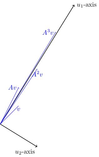
12.05 Here's a picture of the eigenlines (orthogonal to one another because the matrix $A$ is symmetric) and the positions of $v,Av,A^{2}v,\ldots$ . You can see that these vectors get closer and closer to the $u_{1}$ -eigenline (and stretched out in the $u_{1}$ -direction). They move from side to side of this axis because the sign of $\lambda_{2}$ is negative. So $A^{n}v$ gets more and more parallel to $u_{1}$ as $n\to\infty$ .

The vectors A^nv approach the u_1 direction as n goes to infinity

Arnold cat map

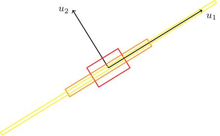
14.26 Here's another nice example, due to Vladimir Arnold. Consider $A=\begin{pmatrix}2&1\\ 1&1\end{pmatrix}$ . This has eigenvalues $\frac{3\pm\sqrt{5}}{2}$ : one of these is bigger than 1, the other is positive but less than 1. Here are the eigenlines, with a square $S$ drawn on (whose sides are parallel to the eigenlines). We also draw $A(S)$ and $A^{2}(S)$ . We can see that it gets stretched in the $u_{1}$ -direction and squashed in the $u_{2}$ -direction (because $\lambda_{1}>1$ and $\lambda_{2}<1$ ). In the limit, $A^{n}(S)$ gets thinner and thinner and closer to the $u_{1}$ -eigenline.

The cat map squashes rectangles in the u_2 direction and stretches them in the u_1 direction

16.40 This is called the Arnold cat map because of the following strange phenomenon. Take an infinite grid of squares in $\mathbf{R}^{2}$ , take a picture of a cat, and put it into every square. Apply $A$ to this grid of cats. The cats will get stretched and squashed in the eigendirections. Pick one of our original squares and look at what's there. We see a bunch of cats all chopped up and stretched and squished back into that square in some way. Now repeat, and repeat. What we see in our square is absolute carnage for a long time. But, amazingly, at some point, we our cat reappears almost identically to how it looked to begin with. This is not because of any periodicity: $A^{n}$ is not the identity for any $n>0$ . This is instead an instance of "Poincaré recurrence": a phenomenon in dynamical systems which goes way beyond anything we're discussing in this course.